Linear Regression
Started: ;
Posted: ;
Last updated:
TL;DR
- When choosing between linear regression models, look to the respective objective functions and match these to your assumptions about the data.
- The classic linear model, Ordinary Least Squares (OLS), is the Best (minimum variance) Linear Unbiased Estimator (BLUE) under the Gauss-Markov assumptions.
- OLS and related linear estimators are computationally efficient, often admitting closed-form solutions, and highly interpretable.
- More flexible models (e.g., neural networks) can better capture complex relationships and improve predictive accuracy at the cost of interpretability and efficiency.
Table of Contents
Click the header to navigate to that section:
1.What is Linear Regression?
Linear regression is a set of techniques used to estimate a linear relationship that best predicts an outcome based on observed data.
But what does it mean to “best” predict? How do we define “best”?
The answer lies in the objective function used to estimate the model.
1.1.The Objective Function
The objective function is a mathematical expression that measures how well a model fits a set of data. The goal of the regression algorithm is to choose model parameters that optimize this function.
Different types of linear regression differ in the objective functions they optimize.
Two examples are:
- Ordinary Least Squares (OLS) Regression, whose objective function is the sum of squared vertical prediction errors.
- Total Least Squares (TLS) Regression, whose objective function is the sum of squared orthogonal prediction errors.
Figure 1 illustrates vertical residuals used in the OLS objective function and orthogonal residuals used in the TLS objective function. The residuals are shown in relation to the respective OLS and TLS lines of best fit for the same 10 data points. These lines of best fit represent the model solutions which optimize the respective objective functions.
Figure 1.OLS Calculates Residuals Along y; TLS, Across Dimensions, in Equal Proportion


Now that we better understand the objective functions that define our linear regression models, how do we know which objective function and model we should choose?
1.2.Choosing a Regression Model
Choosing the correct regression model depends on knowing, or reasonably assuming, properties of the data.
Properties we consider include:
- Random sampling of data from the population of interest,
- Exogeneity (the absence of systematic error once predictors are accounted for),
- Homoskedasticity (constant variance of errors given predictors).
Different regression models, by means of their objective functions, correspond to different assumptions about these and other properties of the data.
Take, for example, the choice between OLS and TLS.
1.3.Example: OLS vs. TLS
The relevant underlying assumption that differentiates OLS and TLS is:
- In OLS, we assume that there is noise in the outcome variable, but not in the predictor variables.
- In TLS, we assume that there is noise in both and variables, of comparable scale.
To visualize the performance of these two models with respect to the nature of the data, I simulate an example where the underlying relationship between and is given by:
In practice, we do not observe the true variables and , but noisy measurements and .
OLS should be used when we assume that there is noise in , but not in .
For example, when our observed values are of the form:
TLS should be used when there is noise not only in , but also in , at comparable scale. For example, when:
Figure 2 illustrates how OLS and TLS behave relative to the underlying relationship, , for a random sample of 100 data points where , and , for .
Figure 2.OLS Performs Best When There is No Error in Observed y; TLS, When Error is Proportionate Across Observed Variables


This progression highlights a key assumption underlying OLS: noise is confined to the outcome variable. As measurement error in increases, this assumption breaks down, and the OLS estimate (the slope of the OLS line in Figure 2) becomes increasingly biased towards zero ("attenuation bias").
Thinking back to the OLS objective function, it is intuitive that OLS will become suboptimal as noise in increases. OLS minimizes the sum of squared vertical (calculated along the y-axis) residuals. It does not account for noise along the x-axis.
In contrast, TLS accounts for noise in both variables, allowing it to recover the true relationship more accurately as the magnitude of the error in approaches the magnitude of the error in .
Thinking back to the TLS objective function, this outcome is also intuitive. TLS minimizes the sum of squared orthogonal residuals, thereby accounting for proportionate deviations in both and .
The key takeaway is that the choice of regression method—and the objective function it optimizes—should be driven by assumptions about the data. In this example, OLS assumes noise is confined to , while TLS assumes noise is equally distributed in all directions.
2.Ordinary Least Squares (OLS)
In this section, we focus on OLS linear regression. OLS is widely used in industry and research because it is computationally efficient and highly interpretable.
We begin by discussing the OLS closed-form solution (the secret to its computational efficiency), then move on to three toy examples: a univariate model of country-level GDP per capita on life expectancy at birth, and two improved multivariate models for life expectancy at birth.
2.1.OLS Closed-Form Solution
Most data scientists will not need to derive (or even know) the mathematical solution to OLS. In practice, statistical packages such as statsmodels, in Python, already know the solution, and use it on our behalf.
However, understanding the structure of the solution is useful. In particular, OLS admits a closed-form solution, which makes it computationally efficient compared to many other models that require iterative optimization.
This is the key takeaway.
In the next section, we plug in real World Bank data on GDP per capita () and life expectancy at birth () to derive a simple, univariate model predicting the latter.
2.2.Univariate OLS Example: GDP vs Life Expectancy
Using 2023 life-expectancy-at-birth and 2024 GDP-per-capita data from the World Bank (the latest available dataset as of March 2026), we estimate the following univariate OLS model:
The model coefficients can be interpreted as follows:
- When the country-level GDP per capita is zero, life expectancy at birth is predicted to be just under 36 years.
- For every 10x increase in GDP per capita, there is a roughly 10 year increase in life expectancy at birth.
Figure 3 plots the model line of best fit against the scatter plot of country data points. A subset of data points falling above, near, and below the line are labeled.
Figure 3.A 10x Increase in GDP per Capita is Associated with a Roughly 10 Year Increase in Life Expectancy


While we can clearly see that a country’s GDP per capita is positively correlated with resident life expectancy at birth, we also see that the former is a blunt tool for predicting the latter.
For example, using this model, we would overpredict the life expectancy at birth in the U.S. at 83 years when it is really 78 years. In contrast, we would underpredict the life expectancy at birth in French Polynesia at 78 years, when it is really 84 years.
Some additional factors we can reasonably assume influence life expectancy at birth, which could help to explain the differing life expectancies in French Polynesia and the U.S., include:
- Widespread access to quality healthcare
- Fitness and nutritional education
- Access to nutritious foods
These factors may themselves be more prevalent in wealthier countries, which would positively bias the univariate OLS coefficient for GDP per capita, making it seem as though GDP per capita has a greater influence on life expectancy than it actually does.
We expand on this point in the following section, in which we introduce two new variables to our simple model.
2.3.Multivariate OLS Examples: Improved Models for Life Expectancy
In this section, I estimate three different OLS models:
- Model 1 is the same univariate model that was estimated in the previous section.
- Model 2 includes a second explanatory variable: the measles immunization rate among children ages 12-23 months, a proxy for widespread access to healthcare.
- Model 3 includes a third explanatory variable: the rate of secondary school enrollment, a proxy for fitness and nutritional education.
The measles immunization rate and secondary school enrollment variables are both published by the World Bank. For each country included in the model, we use the latest-available data between 2020 and 2025, as of March 2026.
Table 1 shows the outputs of these models.
Table 1.Comparison of OLS Models:
| Dependent variable: Life Expectancy at Birth (Years) | |||
| GDP Only | + Immunization | + Education | |
| (1) | (2) | (3) | |
| Log10 GDP per Capita (2015 USD) | 9.86*** | 9.03*** | 7.52*** |
| (0.43) | (0.50) | (0.73) | |
| Immunization (%) | 0.08*** | 0.07*** | |
| (0.02) | (0.02) | ||
| Secondary School Enrollment (%) | 0.05*** | ||
| (0.02) | |||
| Intercept | 35.66*** | 31.58*** | 34.49*** |
| (1.66) | (1.92) | (2.37) | |
| Observations | 192 | 181 | 155 |
| R2 | 0.74 | 0.75 | 0.75 |
| Adjusted R2 | 0.74 | 0.75 | 0.75 |
| Residual Std. Error | 3.69 | 3.56 | 3.49 |
| F Statistic | 535.33*** | 274.25*** | 152.64*** |
| Notes: | *p<0.1; **p<0.05; ***p<0.01 | ||
| Standard errors in parentheses. GDP per Capita is log transformed with base 10. Immunization refers to measles vaccination rates among children ages 12–23 months. Data are the latest available as of March 2026, with GDP per capita data from 2024 and life expectancy data from 2023. Immunization and secondary school enrollment data are the latest available between 2020 and 2025, depending on the country. | |||
The coefficients of model 3, the most comprehensive model, can be interpreted as follows:
- For a given country whose measles immunization rates and secondary enrollment rates are held constant, a 10x increase in GDP per Capita is associated with a 7.5 year increase in life expectancy at birth.
- For a given country, whose GDP per capita and secondary enrollment rates are held constant, a 10% increase in the measles immunization rate is associated with a nearly one (0.7) year increase in life expectancy at birth.
- For a given country, whose GDP per capita and measles immunization rates are held constant, a 10% increase in the secondary school enrollment rate is associated with a 0.5 year increase in life expectancy at birth.
- For a country whose GDP per Capita is $1 (log10 GDP per Capita = $0), whose measles immunization rate is 0%, and whose secondary school enrollment rate is 0%, predicted life expectancy at birth is 34.5 years.
Notably, with the inclusion of each additional explanatory variable in models 2 and 3, the estimated effect of GDP per Capita on life expectancy declines. This decline is illustrated in Figure 4.
Figure 4.Adding Controls Reduces the Estimated Effect of GDP per Capita on Life Expectancy


The changing estimated effect shown in Figure 4 illustrates omitted variable bias. That is, in model 1, when relevant immunization and education explanatory variables are excluded from our model and are correlated with the included explanatory variable, as demonstrated in Figure 5, the included variable, GDP per Capita, will have a biased coefficient.
Figure 5.Log GDP per Capita, Immunization, and Secondary Enrollment are Positively Correlated
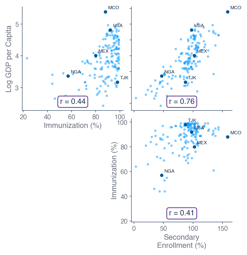
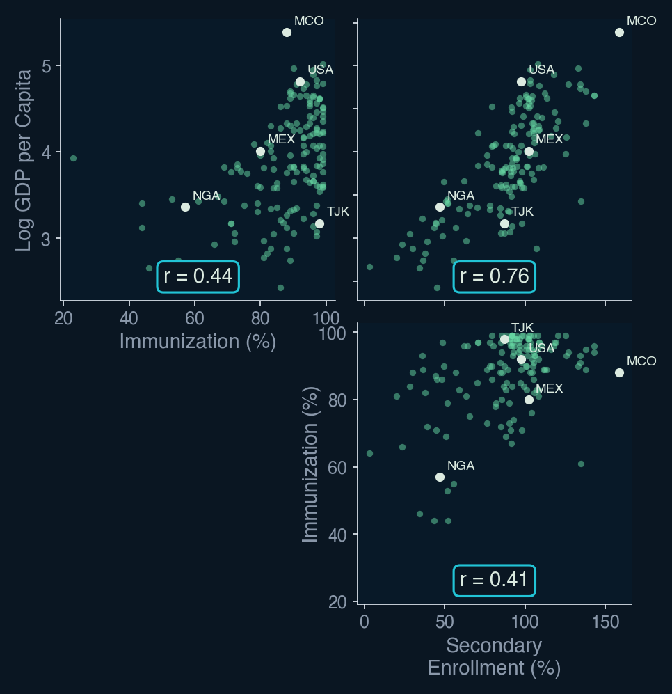
Figure 5 confirms what we previously predicted: that immunization and secondary school enrollment rates tend to be higher in wealthier countries. Similarly, countries with higher immunization rates tend to have higher secondary school enrollment rates.
These positive correlations help us understand the direction of the omitted variable bias observed in Figure 4. Because the omitted variables for immunization and enrollment rates are both positively correlated with log GDP per capita, excluding the enrollment variable from model 2 and excluding both enrollment and immunization variables from model 1 causes variation in life expectancy that would be attributed to immunization and/or education rates to instead be attributed to GDP per capita. This positively biases the GDP per capita coefficient, which moves from 9.86 in model 1, when the immunization and enrollment variables are excluded, to 7.52 in model 3, when these variables are included.
Looking back at Table 1, we can see that the immunization coefficient in model 2 was also positively biased when excluding the secondary school enrollment variable (moving from .08 in model 2 to .07 in model 3). Again, the direction of this bias makes sense considering that immunization rates and enrollment rates are also positively correlated with one another.
In summary, while the simple, univariate model in Figure 3 tells a compelling story (i.e., that life expectancy tends to be higher in wealthier countries), it does not tell the full story. Evidently, quality-of-life factors which are themselves associated with country-level wealth, such as access to quality healthcare and education, play a roll in advancing life expectancy at birth for a given country's newborns.
Building an accurate model, from which we can reliably extract insights, depends on a deep apriori understanding of what factors reasonably influence the outcome variable and on the availability and reliability of data that speak to those factors.
This issue of variable selection is one of multiple "make-it-or-break-it" modeling decisions we discuss in detail in the following section.
3.When OLS Fails and What to Do About It
We have already discussed two failure modes of OLS above.
- In Section 1.3: Example: OLS vs. TLS, we saw how the OLS coefficient became increasingly biased toward zero ("attenuation bias") as we increased noise in the explanatory variable.
- In Section 2.3: Multivariate OLS Examples: Improved Models for Life Expectancy, we saw how the exclusion of relevant variables from the OLS model biased the coefficient of included variables that were correlated with the excluded variables ("omitted variable bias").
Unfortunately, there are many more potential "failure modes" of OLS that can bias our coefficients and/or standard errors. Biased coefficients and/or standard errors undermine inference — the process of using sample data to reliably answer questions about the wider population or the underlying relationship between the predictor(s) and the outcome variable.
Fortunately, we can explore these potential failure modes systemmatically by means of the six assumptions of OLS.
3.1.The Six Assumptions of OLS
In this section, we define the six assumptions of OLS in the context of a multivariate, cross-sectional OLS model.
If you are already familiar with these, feel free to skip ahead to Section 3.2: How to Diagnose OLS Assumption Violations.
OLS Assumption #1: Linearity in model parameters
The model is linear in its parameters. This assumption is embedded in the OLS objective function and, therefore, in the derivation of the OLS closed-form solution.
That said, the model does not have to be linear in its variables. For example, is valid because it remains linear in , even though it includes a nonlinear transformation of .
OLS Assumption #2: No perfect collinearity
No predictor is a perfect linear combination of other predictors. For example, , where and are both included predictors, violates perfect collinearity. When this occurs, the OLS closed-form solution does not exist.
Furthermore, no predictor is a constant. There must be variation in each predictor's values in order to analyze the effect of a change in the predictor on the change in the outcome variable.
OLS Assumption #3: Random sampling
The data are independently and identically distributed (i.i.d.) draws from the population of interest.
This assumption allows sample averages to approximate population expectations via the Law of Large Numbers and underpins large-sample inference via the Central Limit Theorem.
For reference:
The Law of Large Numbers (LLN) states that, for a sequence of i.i.d. random variables with finite mean, the sample average converges in probability to the true population mean as the sample size increases. Formally:
The Central Limit Theorem (CLT) states that for a sequence of i.i.d. random variables with finite mean and variance, the standardized sample average converges in distribution to a standard normal distribution as the sample size increases. Formally:
OLS Assumption #4: Exogeneity (zero conditional mean)
Errors are exogenous. Put simply, this means there is nothing in the error term that is systematically related to model predictors.
Exogeneity can take on multiple formal definitions (i.e., stricter or weaker definitions of exogeneity) depending on the context. For the case of cross-sectional OLS, exogeneity is defined by an expected error value of zero conditional on the predictors (zero conditional mean):
Both of the failure modes we discussed earlier (error in and omitted variables) led to OLS violations of exogeneity.
When exogeneity is violated, model coefficients are biased. In the cases we discussed earlier, the specific types of bias were attenuation bias and omitted variable bias, respectively.
OLS Assumption #5: Homoskedasticity
Errors have constant variance conditional on the predictors ("homoskedasticity"). Homoskedasticity is required for accurate OLS standard errors and, therefore, accurate t-statistics and hypothesis testing.
This assumption is not required for unbiasedness, but it ensures OLS is the most efficient (minimum variance) linear unbiased estimator.
When homoskedasticity is violated (i.e., errors are heteroskedastic), the usual OLS standard errors are inconsistent and must be replaced with heteroskedasticity-robust (Huber–White) standard errors to obtain asymptotically valid inference.
Alternatively, if the form of heteroskedasticity can be correctly specified, Weighted Least Squares (WLS) can be used to obtain more efficient estimates and valid standard errors. (See: Section 4.1: WLS, GLS, and FGLS.)
OLS Assumption #6: Error normality
The error, conditional on , is normally distributed.
Normality is required for inference (e.g., t-tests and confidence intervals) at small sample sizes (as a rule of thumb, ).
That said, under standard regularity conditions where are jointly i.i.d., with finite second moments, and for some positive definite matrix , the OLS estimator is asymptotically normal even when the errors are not. This means that for large (relative to the number of predictors), we use the usual t-statistic, but compare it to the standard normal (z) distribution
Table 2 summarizes each of the OLS assumptions along with what they "get" us in terms of model structure, unbiasedness, efficiency, and large- and small-sample inference.
Table 2.Summary of OLS Assumptions and Why They Matter
| Assumption | Role | Why it matters |
|---|---|---|
| 1. Linearity in parameters | Model structure | Ensures OLS is well-defined |
| 2. No perfect collinearity | Model structure | Ensures coefficients are identifiable |
| 3. Random sampling | Large-sample inference | Ensures observations are i.i.d., underpinning the LLN (consistency) and the CLT (asymptotic normality) |
| 4. Exogeneity | Unbiasedness | Ensures estimates target true parameters (unbiased in small samples; consistent in large samples) |
| 5. Homoskedasticity | Efficiency | Ensures OLS is the most efficient (minimum variance) linear unbiased estimator |
| 6. Error normality | Small-sample inference | Enables exact small-sample t-tests |
Understanding these, we may still choose to use OLS for its unbiasedness property when assumptions 1-4 are satisfied, even if homoskedasticity is violated. In this case, we could substitute heteroskedasticity-robust standard errors for the classical OLS standard errors.
However, if exogeneity fails, OLS estimates are biased and inconsistent. In this case, OLS may still be useful for describing correlations, but it cannot be given a causal interpretation, and standard inference on the structural parameters of interest is invalid. Alternative methods (e.g., instrumental variables) are required.
But first, how do we know when these assumptions are violated?
3.2.How to Diagnose OLS Assumption Violations
Some OLS violations are diagnosable through statistical testing. Others require a solid understanding of the underlying subject matter and data quality to diagnose. Common statistical and reasoning diagnostic methods corresponding to each of the OLS assumptions are summarized in Table 3.
Table 3.Methods for Diagnosing OLS Assumption Violations
| Assumption | Reasoning / Design Checks (Before Estimation) | Empirical Diagnostics (After Estimation) |
|---|---|---|
| 1. Linearity in parameters |
|
|
| 2. No perfect collinearity |
|
|
| 3. Random sampling |
|
|
| 4. Exogeneity (zero conditional mean) |
|
|
| 5. Homoskedasticity |
|
|
| 6. Error normality |
|
*Both of these tests can reject normality trivially in large samples. |
When working on an empirical project, much of the 'thinking through' potential violations should happen before you run your first regression. I discuss each of the assumptions, and the stages at which you can think through potential issues, below.
-
Linearity in parameters and model structure should be the first consideration when starting a new project, as misspecification at this stage invalidates everything that follows. Before running a regression, think about the functional form: should any variables enter in logs? Are there theoretical reasons to expect threshold or interaction effects? These decisions should be guided by domain knowledge and verified by post-hoc testing.
-
No perfect collinearity should fall naturally from careful variable selection. You should avoid including redundant dummy variables or mechanically related variables (e.g., shares that sum to one).
-
Random sampling should be assessed before estimation as well. How was the sample constructed? Are there obvious sources of selection bias? These questions are answered by understanding your data collection process.
-
Exogeneity is the most consequential assumption and the hardest to verify empirically — there is no test that can definitively establish it. This is where subject matter knowledge does the most work. Think carefully about omitted variables, reverse causality, and measurement error before running your first regression. Post-estimation tools — sensitivity analyses for confounding variables and specification tests like the Hausman test — can probe robustness, but they cannot substitute for a credible identification argument.
-
Homoskedasticity can be assessed after estimation via residual plots and formal tests.
-
Error normality is the least urgent assumption to diagnose in most applied settings. In large samples, the CLT renders it largely irrelevant for inference, as discussed in Section 3.1: The Six Assumptions of OLS. It matters primarily in small samples where you are relying on exact distributional results. In this case, it can be assessed post-estimation via Q-Q plots or formal tests.
Once we have identified issues (again, often by thinking through the underlying subject area), there are multiple ways to address them. I discuss these "next steps" systematically in the next section.
3.3.What to Do When OLS Assumptions Are Violated
Not all assumption violations are equally serious, and the appropriate response depends on which assumption is violated and why. Here, we discuss remedies as they apply to violations of each assumption.
-
Linearity in parameters. If residual plots or the RESET test suggest misspecification, the fix is usually a transformation of variables rather than abandoning OLS entirely. Taking logs of skewed variables (e.g., income) is often theoretically motivated and linearizes many common relationships. Polynomial terms or piecewise linear splines can accommodate threshold effects. Interaction terms allow the effect of one variable to depend on another. In more severe cases — where the functional form is genuinely unknown — nonparametric or semiparametric methods (read: not OLS) may be warranted, at the cost of interpretability.
-
No perfect collinearity. If perfect collinearity exists, OLS cannot be estimated. The fix is to drop one of the collinear variables, which is often the right thing to do on conceptual grounds anyway (e.g., dropping one category of a set of dummies). Near-multicollinearity is a different matter: OLS remains unbiased, but standard errors become large. The appropriate response is usually not to drop variables arbitrarily, as this risks omitted variable bias. Instead, consider whether a larger sample size would help (assuming it is feasible to collect more data) or if the imprecision is an honest reflection of the limits of what the data can tell you.
-
Random sampling. If the sampling process is known and based on observables, sample weighting (e.g., weighted least squares) can restore representativeness. In cases of clustered observations — where units within groups share common shocks (e.g., students within the same school, sharing the same teachers)— the standard fix is to use cluster-robust standard errors, which account for within-cluster correlation. If the selection mechanism is unknown or related to unobservables, the problem is more severe and will violate exogeneity.
-
Exogeneity. This is the most serious violation and the hardest to fix. If exogeneity fails, OLS estimates are biased and inconsistent, and no amount of standard error adjustment will rescue the point estimates themselves. The appropriate remedy depends on the source of the violation:
- Selection bias: If sample inclusion is related to the outcome (e.g., estimating wages using a dataset of only employed individuals), you can apply Heckman selection models that account for the probability of being included in the sample.
- Omitted variable bias: Include the omitted variable if it is observable. If not, consider whether a proxy variable is available.
- Reverse causality: Instrumental Variable (IV) estimation can break the simultaneity, provided a valid instrument exists — one that affects , and affects only through .
- Measurement error in regressors:
IV can also address classical measurement error (attenuation bias),
again requiring a valid instrument (in this case, an instrument that does not also suffer from measurement error.)
Note. As discussed in Section 1.3: Example: OLS vs. TLS, TLS can be used when there is reason to believe that the measurement error in is of similar magnitude to the measurement error in . Similarly, weighted TLS may be used when you have a good estimate for the relative magnitude of measurement errors in compared to . This is seldom known in practice.
In summary, when exogeneity is violated, the goal is to replace an untestable assumption with a more credible one.
-
Homoskedasticity. This is the most straightforward violation to address. If heteroskedasticity is present, OLS remains unbiased and consistent — the problem is purely with inference. The standard fix is to use heteroskedasticity-robust standard errors, which are valid asymptotically without requiring homoskedasticity. In the presence of both heteroskedasticity and clustering, cluster-robust standard errors address both simultaneously.
-
Error normality. In large samples, non-normal errors generally require no remedy: under standard regularity conditions, OLS estimators are asymptotically normal even when the error distribution itself is not. In small samples where exact inference matters, sometimes transforming the outcome variable can help if the non-normality is driven by skewness.
The overall message is that violations of assumptions 1–3 and 5–6 are generally manageable with well-understood techniques. Violations of assumption 4 (exogeneity) are categorically more serious, as they compromise the estimator itself rather than just its precision or distributional properties.
4.Building on Top of OLS
So far, we have discussed classical, cross-sectional OLS in depth. In this section, we discuss two families of extensions to OLS: a family of reweighting extensions (WLS, GLS, and FGLS) and a family of regularization methods (Ridge, Lasso, and Elastic Net). For each, we will discuss their objective functions and why classical OLS is nested within these as a special case. We also discuss why these modifications are useful and when they should be employed.
4.1.WLS, GLS, and FGLS
Recall from Section 3.1: The Six Assumptions of OLS that a violation of homoskedasticity (assumption 5) leaves OLS unbiased but no longer the most efficient (minimum variance) linear unbiased estimator. In Section 3.3: What to Do When OLS Assumptions Are Violated, we discussed one fix: heteroskedasticity-robust standard errors. This fix preserves the OLS point estimates and corrects inference, but it does not improve efficiency.
Weighted Least Squares (WLS), Generalized Least Squares (GLS), and Feasible Generalized Least Squares (FGLS) take a different approach. Rather than correcting standard errors after the fact, they reweight observations during estimation in order to produce coefficient estimates that are themselves efficient under heteroskedasticity (WLS, GLS, FGLS) or under both heteroskedasticity and correlated errors (GLS, FGLS).
Each of these estimators can be viewed as a generalization of OLS in which the equal weighting of observations is replaced by a weighting that reflects the structure of the errors.
- Weighted Least Squares (WLS)
WLS modifies the OLS objective function by assigning each observation its own weight:
The intuition is straightforward: when some observations are noisier than others, we want to down-weight them so that they exert less influence over our coefficient estimates. The efficiency-optimal choice of weights is , where is the conditional error variance for the th observation. Observations with larger error variance receive smaller weights, and vice versa.
Notice that when all are equal—as is the case under homoskedasticity, where for all —WLS reduces exactly to OLS. In this sense, OLS is the special case of WLS in which every observation is weighted equally.
WLS should be used when the form of heteroskedasticity is known—for example, when domain knowledge tells us that error variance scales with a known function of a predictor. In practice, this assumption is rarely satisfied, which motivates FGLS (#3, below).
- Generalized Least Squares (GLS)
GLS extends WLS to the more general setting where errors may be both heteroskedastic and correlated across observations. Correlated errors arise often in practice — most familiarly in time series data, where errors in adjacent periods are typically serially correlated, but also in clustered data, where observations within a group (e.g., students in the same school) share unobserved shocks. In these cases, GLS uses the structure of to recover efficiency.
The GLS objective function is:
Where is the (assumed known) conditional variance-covariance matrix of the errors.
The GLS objective function nests both OLS and WLS:
- When (homoskedastic, uncorrelated errors), GLS reduces to OLS.
- When is diagonal but not proportional to (heteroskedastic, uncorrelated errors), GLS reduces to WLS with .
- When has non-zero off-diagonal entries (correlated errors), GLS captures structure that WLS cannot.
When is correctly specified, GLS is the Best Linear Unbiased Estimator under a generalized version of the Gauss-Markov assumptions—it has the lowest variance among all linear unbiased estimators.
In practice, however, is rarely known, which motivates FGLS.
- Feasible Generalized Least Squares (FGLS)
FGLS addresses the practical problem that is almost never known by estimating it from the data and then plugging the estimate into the GLS formula. The procedure has two steps:
- Estimate the model by OLS and recover the residuals .
- Use to construct an estimate , then compute .
The way is constructed depends on what is assumed about the structure of the errors. For example, if the errors are assumed heteroskedastic with variance depending on the predictors, might be estimated by regressing on . If the errors are assumed to follow an AR(1) process, in which each period's error is correlated with the previous period's error, the autocorrelation parameter can be estimated from the residuals and used to construct a Toeplitz-structured whose entries decay geometrically with the distance between observations.
Table 4 summarizes the relationships between OLS, WLS, GLS, and FGLS.
Table 4.Summary of OLS, WLS, GLS, and FGLS
| Estimator | Assumed Error Structure | When to Use |
|---|---|---|
| OLS | , estimated from residuals | Homoskedastic, uncorrelated errors with unknown but estimable variance; small and large samples |
| WLS | , known | Heteroskedastic, uncorrelated errors with known variance structure |
| GLS | , known | Heteroskedastic and/or correlated errors with known variance-covariance structure |
| FGLS | , estimated from residuals | Heteroskedastic and/or correlated errors with unknown but estimable variance-covariance structure; large samples |
The common thread across WLS, GLS, and FGLS is that each replaces OLS's implicit equal weighting of observations with a weighting derived from the error variance-covariance structure. When that structure is the identity multiplied by a scalar, all three collapse back to OLS. When it is not, they recover efficiency by leveraging information about how the errors behave.
4.2.Ridge, Lasso, and Elastic Net
Recall from Section 3.1: The Six Assumptions of OLS that OLS is unbiased under the Gauss-Markov assumptions. Nonetheless, it can still produce coefficient estimates with high variance. This typically happens in two settings: when predictors are highly (though not perfectly) correlated, and when the number of predictors is large relative to the sample size . In Section 3.3: What to Do When OLS Assumptions Are Violated, we noted that near-multicollinearity inflates standard errors but does not bias OLS, and suggested collecting more data as a remedy. In practice, more data is often unavailable, and large standard errors translate into unstable predictions.
Ridge, lasso, and elastic net take a different approach. Rather than reducing variance by collecting more data, they reduce variance by shrinking coefficients toward zero. This introduces bias in exchange for a reduction in variance, often improving predictive performance (mean squared error) through this bias–variance tradeoff. Each estimator generalizes OLS by replacing the unconstrained minimization of squared residuals with a penalized objective that discourages large coefficient magnitudes. The intercept is left unpenalized.
- Ridge Regression
Ridge modifies the OLS objective function by adding an penalty on the coefficients:
Where is a tuning parameter that controls the strength of the penalty. When , ridge reduces exactly to OLS. As , all coefficients are shrunk toward zero.
The intuition is that, by penalizing the squared magnitudes of the coefficients, ridge prevents any single coefficient from becoming very large in response to noise or near-collinearity in the predictors. Coefficients on correlated predictors are shrunk together rather than allowed to swing in opposite directions to fit small fluctuations in the data.
Ridge should be used when many predictors are expected to contribute small to moderate effects, when predictors are highly correlated, or when is large relative to .
For example, consider a risk score that predicts an individual's genetic predisposition to a complex trait, such as the risk of type 2 diabetes, from hundreds of thousands of genetic markers. This is a setting where prediction is unambiguously the goal: the score is used to flag individuals at elevated risk, not to make causal claims about any single genetic marker. In other words, we can reasonably sacrifice OLS' unbiasedness property in favor of Ridge's biased, but lower variance predictions.
Three features of this setup make ridge an appropriate choice:
- The genetic architecture of most complex traits is highly polygenic: i.e., the trait is influenced by many thousands of variants, each contributing a tiny effect, rather than a small number of variants with large effects.
- Neighboring genetic markers are often correlated with one another.
- The number of data points (, often in the hundreds of thousands) vastly exceeds the number of individuals in the training sample (, often in the tens of thousands), so is singular and OLS is undefined. Ridge shrinks all predictor coefficients toward zero together, preserving the polygenic signal and producing more accurate predictions on new individuals than if we were to simply select some of the predictors to the exclusion of others.
Crucially, the signal is dense rather than sparse: we expect virtually all of the candidate variants to be contributing something, even if very little. This is what tips the balance toward ridge over methods that perform variable selection — there is no sparse subset to identify, and zeroing out variants would discard genuine signal.
Because ridge shrinks coefficients smoothly toward zero but never sets them to exactly zero, it does not perform variable selection — every predictor remains in the model.
- Lasso Regression
Lasso (Least Absolute Shrinkage and Selection Operator) modifies the OLS objective function by adding an penalty on the coefficients:
Where and again controls the strength of the penalty. As with ridge, recovers OLS and shrinks all coefficients toward zero.
The key practical difference between lasso and ridge is that the penalty has corners at zero. As a result, for sufficiently large , lasso will set some coefficients to exactly zero, effectively performing variable selection alongside estimation. Ridge, in contrast, only ever shrinks coefficients toward zero asymptotically.
As with ridge, OLS is the special case of lasso in which the penalty is set to zero.
Lasso should be used when you suspect that only a subset of the potential predictors is truly relevant — that is, when the true coefficient vector is sparse. Because lasso produces models with fewer non-zero coefficients, it often yields more interpretable models than ridge.
For example, suppose a hospital wants to identify which recently discharged patients are at high risk of being readmitted within 30 days, so it can target follow-up interventions toward them. The hospital's records database contains hundreds of predictors per patient: demographic information (age, sex, insurance type), admission diagnosis, length of stay, recent lab values, comorbidities, and prescribed medications, among others. As in the case of the genetic risk score, prediction — not inference on any single coefficient — is the goal, so we are again willing to accept some bias in our coefficient estimates in exchange for lower variance.
Unlike the genetic risk score case, however, we do not expect every potential predictor to contribute. Two features of this setup make lasso an appropriate choice:
- The truth is plausibly sparse: of the hundreds of potential predictors, we expect only a small subset — likely related to disease severity and specific high-risk comorbidities — to meaningfully drive readmission risk. Most other variables are likely irrelevant.
- The model is intended to support clinical decision-making, where interpretability matters. A model that depends on a handful of identifiable clinical variables is easier for physicians to scrutinize, trust, and act on than one that distributes small weights across hundreds of features.
By setting the coefficients on uninformative predictors to exactly zero, lasso produces a more compact, more interpretable model and avoids the predictive noise that would come from including hundreds of weak or null contributors.
A known limitation of lasso is its behavior with groups of correlated predictors: when several predictors are highly correlated with one another, lasso tends to arbitrarily select one and zero out the others, even when all are relevant. Elastic net was developed to address this limitation.
- Elastic Net
Elastic net combines the and penalties of lasso and ridge:
Where controls the overall strength of the penalty and controls the relative mix of the and components.
The elastic net objective function nests OLS, ridge, and lasso:
- When , elastic net reduces to OLS.
- When , elastic net reduces to ridge.
- When , elastic net reduces to lasso.
Elastic net inherits the variable-selection behavior of lasso (from the component) and the grouping behavior of ridge (from the component). When predictors are correlated, elastic net tends to select or drop them together rather than arbitrarily picking one, which makes it well-suited to settings with groups of correlated relevant predictors — common in text data, and other high-dimensional applications.
Table 5 summarizes the relationships between OLS, Ridge, Lasso, and elastic net.
Table 5.Summary of OLS, Ridge, Lasso, and Elastic Net
| Estimator | Penalty Term | When to Use |
|---|---|---|
| OLS | None | Low-dimensional setting with uncorrelated predictors and unbiasedness as the priority |
| Ridge | Many small-to-moderate effects, highly correlated predictors, or large relative to ; no variable selection desired | |
| Lasso | Sparse true coefficient vector; variable selection desired; predictors not strongly grouped | |
| Elastic net | Groups of correlated, relevant predictors; variable selection desired with grouping behavior |
The common thread across ridge, lasso, and elastic net is that each augments the OLS objective function with a penalty on coefficient magnitudes. When the penalty is set to zero, all three collapse back to OLS. When the penalty is active, each accept some bias in exchange for a reduction in variance — and, in the case of lasso and elastic net, also performs variable selection.
5.Beyond Linear Regression
Linear regression is a foundational method within supervised machine learning. As we have seen above, the resulting model can then be used to make predictions on new, unseen data.
Linear regression remains widely used because it is interpretable and computationally efficient. However, more complex models can capture nonlinear relationships and interactions between variables, often improving predictive performance at the cost of interpretability.
A range of other supervised machine learning models build on these ideas in different ways, varying in how they define prediction error and how they control model complexity. Common examples include:
- Logistic Regression
- K-Nearest Neighbors (KNN)
- Support Vector Machines (SVM)
- Classification
- Regression (SVR)
- Decision Trees
- Random Forest
- Boosting methods (e.g., XGBoost / LightGBM)
- Neural Networks
- Feedforward / Deep Neural Networks
- Convolutional Neural Networks (CNNs)
- Transformers / Large Language Models (LLMs)
Each of these approaches offers different strengths depending on the structure of the data, the importance of interpretability, and the desired predictive performance.
I will discuss these models in more detail in future blog posts.